Real-Time Elastic Deformation Tracking of a Flexible Skin-Mounted Lattice
A monocular CV system that tracks elastic deformation of a 4×4 flexible silicone lattice adhered to skin, separating per-node elastic displacement from rigid-body limb motion to infer subsurface muscle activity, at 30 fps, using a single USB webcam and no contact instrumentation.
Andrew Thompson
Motivation
A flexible lattice adhered to skin deforms visibly as underlying muscles contract and relax. Tracking this deformation with a standard webcam gives a dense, spatially-resolved strain field that can be correlated with specific muscle groups, without gel, wiring, or clinical hardware.
The core challenge is separating elastic deformation (strain from muscle activity) from rigid-body motion (the limb translating or rotating as a whole). Both show up as node displacement in image space; the tracker solves this decomposition each frame using an ARAP deformation model and a projective rigid-body subtraction step.
Physical Setup
| Parameter | Value |
|---|---|
| Lattice material | Teal/cyan silicone (EcoFlex 00-30) |
| Grid | 4×4 cells, 5×5 intersection nodes |
| Cell pitch | 15.0 mm (12.5 mm hole + 2.5 mm bar) |
| Camera | USB webcam, 1280x720, 30 fps |
| Depth sensor | None |
Status
This is an active, ongoing personal research project, not tied to any lab or employer. The system runs in real time on a standard webcam at 30 fps and produces per-node displacement and per-triangle strain/stress estimates suitable for downstream gesture classification, control mapping, or biomechanical analysis.
Technical Deep-Dive: Architecture, Math, and Engineering Challenges
System Architecture
Five ROS 2 nodes communicate via typed messages. The tracker processes every camera frame at 30 fps; the SAM2 segmenter publishes masks asynchronously at 3-7 fps.
| Stage | Node | Output topic |
|---|---|---|
| 1. SAM2 segmentation | lattice_segmenter_node.py |
/lattice_mask |
| 2. H-initialisation from mask hull | deformation_tracker_arap_node |
internal |
| 3. Cell centroid detection | ↑ | internal |
| 4. KLT optical flow reconciliation | ↑ | internal |
| 5. ARAP deformation solve | ↑ | internal |
| 6. Rigid-body subtraction | ↑ | /deformation_field_arap |
| 7. Strain & stress computation | ↑ | /deformation_field_arap |
| Diagnostics | ↑ | /tracker_diagnostics_arap |
Stage 1 — SAM2 Lattice Segmentation
Meta SAM2’s VideoPredictor (Ravi et al., 2024) is initialised from a single user click on the lattice. The model propagates a binary mask frame-to-frame without further input, and resets every 30 frames to prevent GPU memory accumulation, carrying forward the most-recent mask as the next session’s prompt.
The mask has two uses downstream: it provides the convex hull from which \(H_\text{snap}\) is estimated each frame, and it gates centroid detection so that skin texture outside the lattice is never accepted as a lattice cell.
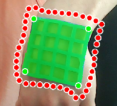 One-click SAM2 initialisation. The model encodes the lattice boundary (red contour) from a single prompt point; green markers indicate the four hull corners extracted for homography estimation.
 The propagated lattice mask in a later frame, tracked automatically from the single initial click with no further user input.
Stage 2-4 — Detection
Cell centroid detection. The Lab \(a^*\) channel is extracted, enhanced with CLAHE (Zuiderveld, 1994), and thresholded via Otsu’s method (Otsu, 1979), which selects the threshold \(t\) that maximizes between-class variance:
\[t^* = \arg\max_t\ \omega_0(t)\ \omega_1(t)\ [\mu_0(t)-\mu_1(t)]^2\]where \(\omega_0,\omega_1\) are the background/foreground pixel-fraction weights and \(\mu_0,\mu_1\) their respective mean intensities. Connected component analysis on the inverted (hole) mask yields one centroid per open cell, computed from each region’s image moments:
\[\bar x = \frac{M_{10}}{M_{00}}, \qquad \bar y = \frac{M_{01}}{M_{00}}\]Node positions are derived from adjacent-cell centroid midpoints along the dominant horizontal and vertical basis vectors \(\hat{h}\), \(\hat{v}\).
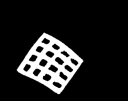 Otsu thresholding of the Lab \(a^*\) channel inside the SAM2 mask. White regions are lattice bars; open cells appear as black holes. Connected component analysis on this mask yields one centroid per cell.
KLT reconciliation. Pyramidal Lucas-Kanade optical flow runs on raw grayscale, not CLAHE, which violates brightness-constancy across frames. The reconciliation rule: if centroid and KLT agree within max_refine_dist, centroid wins; if they disagree, KLT wins; if both fail, the node is marked invalid and ARAP interpolates.
Stage 5 — ARAP Deformation Tracking
The lattice is modelled as a graph \(G = (V, E)\) of 25 intersection nodes. Let \(\mathbf{r}_i \in \mathbb{R}^2\) be the captured rest position of node \(i\) and \(\mathbf{s}_i \in \mathbb{R}^2\) its current position. The As-Rigid-As-Possible (ARAP) energy (Sorkine & Alexa, 2007) minimised each frame is:
\[E_\text{ARAP} = \sum_i \sum_{j \in \mathcal{N}(i)} w_{ij} \left\| (\mathbf{s}_i - \mathbf{s}_j) - R_i(\mathbf{r}_i - \mathbf{r}_j) \right\|^2\]where \(R_i \in SO(2)\) is the best local rotation at node \(i\), found by alternating local and global steps.
Local step — per-node rotation via SVD
With current positions fixed, the optimal rotation at each node minimises the local rigidity energy. This has the closed-form solution:
\[C_i = \sum_{j \in \mathcal{N}(i)} w_{ij} (\mathbf{s}_i - \mathbf{s}_j)(\mathbf{r}_i - \mathbf{r}_j)^T = U \Sigma V^T \qquad \Rightarrow \qquad R_i = VU^T\]Global step — sparse linear system
With rotations fixed, adding observation constraints (weight \(\lambda_i\)) and Tikhonov regularisation to \(E_\text{ARAP}\) and minimising over all node positions gives the linear system:
\[(L + \Lambda) \mathbf{s} = \mathbf{b}\]where \(L\) is the graph Laplacian, and \(\Lambda = \mathrm{diag}(\lambda_i)\) with:
\[\lambda_i = \begin{cases} \lambda_\text{obs} & \text{node } i \text{ observed (centroid or KLT)} \\ \lambda_\text{obs} \cdot \rho & \text{node } i \text{ unobserved (ARAP interpolated)} \end{cases}\]The system is solved with Eigen’s LDLT. Because the system matrix \(A = L + \Lambda\) depends only on the pattern of valid nodes, not their positions, the factorisation is cached and reused across frames whenever the validity pattern is unchanged. At steady state this skips 5 of 6 factorisations per frame.
Unobserved nodes. When cells go dark during rotation, those nodes are held near their \(H_\text{snap}\)-extrapolated positions by a prediction prior with weight \(\lambda_\text{obs} \cdot \rho = 5.0\). Without this anchor a cluster of simultaneously dark cells has 80% of its constraint force from its neighbours, also drifting, and collapses toward its own centroid.
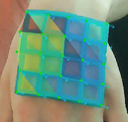 ARAP mesh and strain triangulation during a wrist flexion. Green dots mark directly observed nodes; Delaunay triangles are colour-coded by von Mises stress. The mesh deforms consistently with the underlying surface curvature change.
Stage 6 — Rigid-Body Subtraction via Projective Homography
Raw node displacement \(\mathbf{s}_i - \mathbf{r}_i\) mixes elastic deformation with whole-limb rigid motion. A 4-DOF similarity transform, the natural model for in-plane motion, cannot handle out-of-plane rotation or depth translation in perspective, so those motions appear as false strain.
Instead, a full 8-DOF projective homography \(H_\text{rigid} \in \mathbb{R}^{3 \times 3}\) is fit each frame from the observed nodes via RANSAC (Fischler & Bolles, 1981):
\[H_\text{rigid} = \underset{H}{\arg\min} \sum_{i \in \text{inliers}} \left\| \mathbf{s}_i - \pi\left(H[\mathbf{r}_i; 1]\right) \right\|^2\]where \(\pi(\mathbf{x}) = (x_1/x_3, x_2/x_3)\) is the perspective division. The elastic deformation of each node is then the residual:
\[\mathbf{d}_i = \mathbf{s}_i - \pi\left(H_\text{rigid}[\mathbf{r}_i; 1]\right)\]RANSAC identifies nodes whose motion fits a single projective transform (the rigid body) and flags the rest as potential elastic outliers. An EMA with \(\alpha = 0.7\) is applied to \(\mathbf{d}_i\) across frames to reduce detection noise without adding visible lag.
Stage 7 — Strain Tensor and Plane-Stress Computation
Node deformation vectors \(\mathbf{d}_i\) define a piecewise-linear displacement field over a Delaunay triangulation of the lattice. Within each triangle the small-strain tensor is computed from the constant displacement gradient:
\[\varepsilon = \begin{bmatrix} \varepsilon_{xx} & \varepsilon_{xy} \\ \varepsilon_{xy} & \varepsilon_{yy} \end{bmatrix} = \begin{bmatrix} \partial u_x/\partial x & \tfrac{1}{2}(\partial u_x/\partial y + \partial u_y/\partial x) \\ \tfrac{1}{2}(\partial u_x/\partial y + \partial u_y/\partial x) & \partial u_y/\partial y \end{bmatrix}\]The lattice material is EcoFlex 00-30 silicone (\(E = 69\text{ kPa}\), \(\nu = 0.499\)). Under the plane-stress assumption the Cauchy stress components are:
\[\sigma_{xx} = \frac{E}{1-\nu^2}(\varepsilon_{xx} + \nu \varepsilon_{yy}), \qquad \sigma_{yy} = \frac{E}{1-\nu^2}(\varepsilon_{yy} + \nu \varepsilon_{xx}), \qquad \sigma_{xy} = \frac{E}{1+\nu} \varepsilon_{xy}\]The von Mises effective stress, rendered as a colour heatmap overlaid on the lattice, is:
\[\sigma_\text{vm} = \sqrt{\sigma_{xx}^2 - \sigma_{xx}\sigma_{yy} + \sigma_{yy}^2 + 3\sigma_{xy}^2}\]Valid for small strains (<30%); EcoFlex is hyperelastic at large strains and the linear model underestimates stress in that regime.
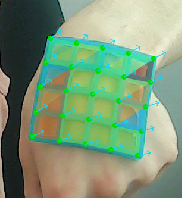 Von Mises stress heatmap during wrist flexion viewed from the dorsal side. Warmer colours indicate higher effective stress concentrated along the bend axis; cooler triangles show relatively unloaded regions.
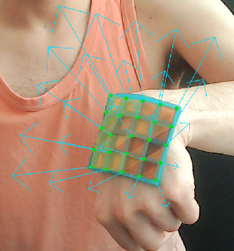 Elastic deformation field when a convex surface is pressed into the lattice center. Material displaced radially outward from the contact point produces the diverging strain pattern shown. Arrows scaled 5x for visibility.
Key Engineering Challenges
D4 symmetry ambiguity. A square 4x4 lattice has four-fold rotational symmetry: the convex hull corners derived from the SAM2 mask can be assigned in any of four cyclic orientations. During wrist rotation the hull degenerates, and the minimum-rotation heuristic for orientation continuity could jump 90 or 180 degrees, flipping the canonical node assignment and producing ~500 kPa von Mises spikes. Fix: reject homography updates where the best cyclic rotation differs from the previous frame by more than 20 degrees, preserving the last stable orientation.
EMA accumulator reset bug. The temporal smoothing filter on deformation was reset every frame to the raw node displacement \(\mathbf{s}_i - \mathbf{r}_i\) before the rigid-subtraction result was blended in. The displayed deformation was therefore 0.7 times the total displacement from rest plus 0.3 times the rigid-subtracted residual, causing strain arrows that grew linearly with how far the arm had moved from the reference position even with zero elastic deformation. Fix: guard the accumulator reset behind a !has_reference flag, so the EMA only initialises at first reference capture and accumulates correctly across subsequent frames.
ARAP mesh condensation during occlusion. When a cluster of adjacent cells goes dark during wrist rotation, unobserved nodes couple primarily to each other via ARAP rigidity with only a small prediction anchor. For a 3x3 occluded cluster the interior node has 80% of its constraint from its drifting unobserved neighbours and only 20% from the \(H_\text{snap}\) extrapolation, so the cluster condenses toward its own centroid. Fix: raise the prediction weight ratio so the \(H_\text{snap}\) anchor becomes the dominant constraint for a fully-unobserved interior cluster.
Performance
| Metric | Value |
|---|---|
| Full pipeline rate | 30 fps at 1280x720 |
| ARAP solve (6 iter, 25 nodes) | ~2 ms |
| Tracked nodes | 25 (5x5 intersection grid) |
| Per-triangle strain tensors | 16 (Delaunay triangulation) |
| LDLT cache hit rate (steady state) | ~83% (5 of 6 iterations/frame) |
References
- Sorkine, O., & Alexa, M. (2007). As-Rigid-As-Possible Surface Modeling. Symposium on Geometry Processing (SGP). Eurographics Digital Library
- Ravi, N., Gabeur, V., Hu, Y.-T., et al. (2024). SAM 2: Segment Anything in Images and Videos. arXiv:2408.00714. arXiv
- Otsu, N. (1979). A Threshold Selection Method from Gray-Level Histograms. IEEE Transactions on Systems, Man, and Cybernetics, 9(1), 62-66. DOI
- Zuiderveld, K. (1994). Contrast Limited Adaptive Histogram Equalization. In Graphics Gems IV (pp. 474-485). DOI
- Fischler, M. A., & Bolles, R. C. (1981). Random Sample Consensus: A Paradigm for Model Fitting with Applications to Image Analysis and Automated Cartography. Communications of the ACM, 24(6), 381-395. DOI
Technologies
C++17 · Python 3 · ROS 2 Humble · OpenCV 4 · Eigen 3 · PyTorch 2 · Meta SAM2 · NumPy · CMake / colcon / ament_cmake